Maxwell’s Equations
The microscopic formulation of Maxwell’s equations are fairly well-known:
However, the formulation we care about (specifically for material simulation) is the macroscopic one:
where $\mathbf J_f = \sigma \mathbf E$.
“What the hell is an H/D field?” These are auxiliary fields.
For computation/analysis purposes it simply suffices to recall that
where $\mathbf M$ is the magnetisation field.
Technically $\mathbf B$ should be called “magnetic flux density” and it differs from the H field in that it takes into account material properties/current distribution.
The unit of $\mathbf B$ is the tesla $\mathrm T$ or in SI units $\text{kg }\text{s}^{-2}\text{A}^{-1}$. The unit of $\mathbf H$ is simply $\text{A m}^{-1}$.
Similarly, the D field is “electric flux density” and is to the E field what the B field is to the H field! In particular,
where $\mathbf P$ is the polarisation field.
Doesn’t matter, we’re just simulating stuff at the end of the day according to some equations anyway.
So we literally just computationally simulate this! (I only know high-school level EM I might be cooked.)
Constitutive Relations
To apply the macroscopic formulation, we need the constitutive relations to connect the auxiliary fields to the ones we’re used to. For linear isotropic materials:
where $\mu=\mu_0(\chi_m+1),\,\varepsilon=\varepsilon_0(\chi_e+1)$, and $\chi_e$/$\chi_m$ are the electric/magnetic susceptibilities of the material respectively.
For at least the start of this project, conductors will not be taken into account, so no need to worry about free current density, polarisation fields, magnetisation, etc.
Materials
Interesting paper called Advanced Material Modelling in EM-FDTD - using as a kind of guide.
EMPossible has a lecture series on Electromagnetic Analysis Using FDTD.
Following also the Purdue 37th lecture Finite Difference Method, Yee’s Algorithm.
Discretisation Setup
Consider only the two curl equations for now (apparent later),
We can write these using the centre-difference/forward-difference approximations to generate our update equations:
Notice how the first update equation lives at $\left( i,j,k;t\right)$ and the second update equation lives at $\left( i,j,k;t+\frac{dt}{2} \right)$. It is important that all terms in each update equation eventually result in those positions and times. This also suggests the order in which these update equations will be executed - first integer times, then half-integer times.
The curl operator mnemonic/definition for generalised coordinates is is:
and thereby expands in the Cartesian system as:
We use this to specify the curl part of the update equation depending on the dimensions the simulation ends up running in.
FDTD Algorithmic Overview
The finite-difference time-domain method is typically used:
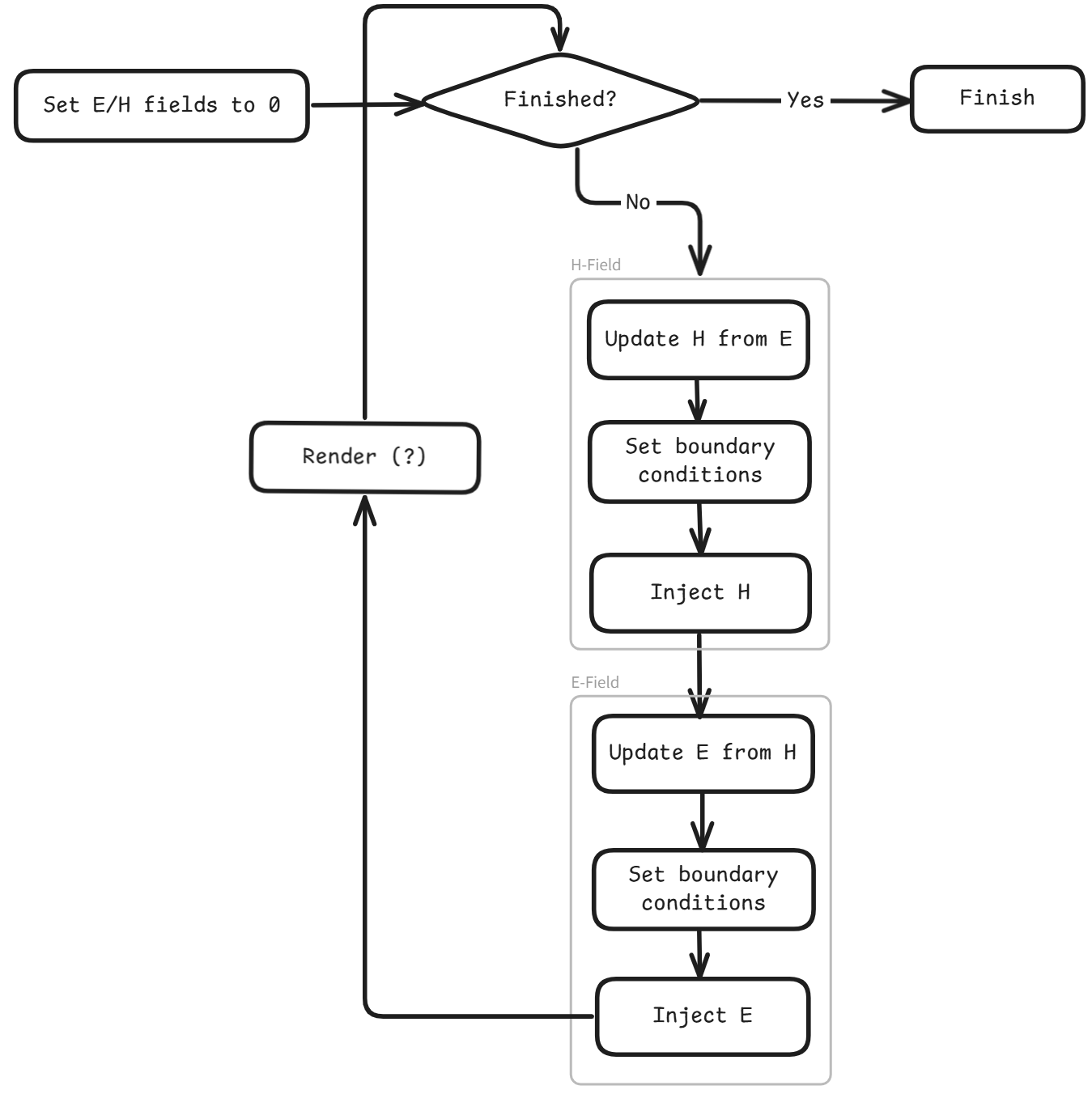
It is easy to see why we do H before E (H takes half steps and is only dependent on $\mathbf E(t)$ and $\mathbf H( t-\frac{dt}{2} )$, while E is dependent on $\mathbf H( t+\frac{dt}{2} )$ as well as the E/H fields at previous times).
For more complex non-isotropic/non-linear materials the constitutive relations need to be baked into the actual simulation (i.e. update B from E, update H from B, update D from H, update E from D, etc.), but this is outside this project scope.
Yee Grid
Motivation
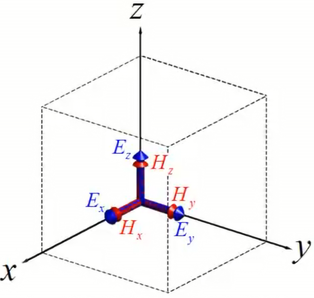
Consider a grid cell. It is standard and tempting to format the grid as shown:
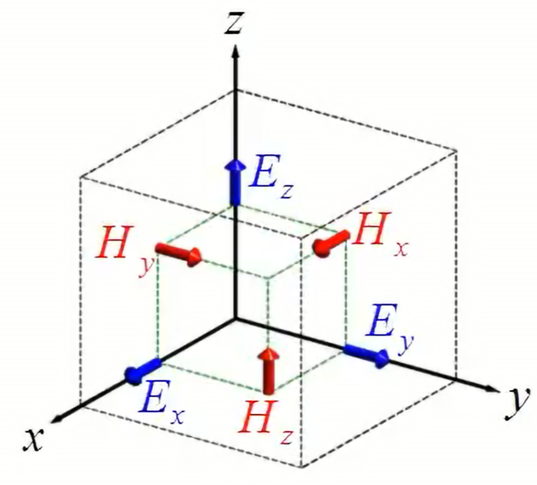
However, this has problems (I’ll take Yee at his word). Basically, stagger the position of the field components, instead of focusing them at a corner:
Turns out this has three major benefits:
- Divergence free field. We only looked at the curl eqns., but turns out that by using this grid, the divergence equations (the two Gauss’s laws) are naturally satisfied - that is, $\nabla \cdot \mathbf B = 0, \, \nabla \cdot \mathbf D = 0$ (assuming $\mathbf J_f,\, \rho_f=0$)
- Emergent boundary conditions. Material boundaries are naturally dealt with (so we don’t have to manually write code to handle the boundary conditions).
- Curl simplification. Notice that with the staggered grid,
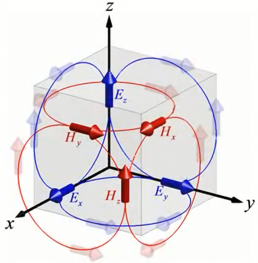
- that is, H fields wrap around E fields and vice versa. This is the exact construction we want in order to approximate curl easily.
For 2D and 1D Yee grids, Maxwell’s equations decouple into two modes (H and E) - i.e. they form two sets of equations (component-wise) with no shared terms between them.
Consequences
Since the H and E field components within one grid cell represent different positions, it means there is phase offset - this needs to be taken into account when injecting sources.
Normalisation
E and H fields differ by several orders of magnitude. To avoid numerical drift, we normalise:
i.e., the curl equations become
where $\varepsilon_r$ and $\mu_r$ are the relative permittivity/permeability constants of the material.