Computational EM - Anisotropy

Motivation

So far the simulation utilises Dirichlet boundary conditions, which gets annoying because of wave reflectance. Hence, want to make an absorbing boundary, known as a perfectly matched layer (PML).

Perfectly Absorbing Boundary

A perfectly absorbing boundary works by absorbing a certain speed of plane wave. This works fine in 1D. However, for 2D, the angle of plane wave affects the speed of incidence ($v\cos\theta$, where $\theta$ is angle of incidence). Therefore, this material is not sufficient.

Uniaxial PML

Fresnel Equations

These equations describe transmittance and reflectance of electromagnetic radiation incident on different media - for $\text{TE}_z$ radiation (i.e. ‘s’ (perpendicularly) polarised light, the $E_z$ mode):

From these two equations we make two observations:

1. We want to set reflectance to be 0, given that we can change $Z_2$.
2. Unfortunately, they are functions of $\theta$. So we need to eliminate $\theta$ somehow to make PML work for all angles of incident light.

Refraction

The refractive index of a material is given by

and can be complex like $\mu_r$ and $\varepsilon_r$ ($n = n'-i\kappa$). The negative of the imaginary part $\kappa$ is known as the extinction coefficient; how quickly the wave decays.

N.B. Notice how we write $n=n'-i\kappa$ instead of $n=n'+i\kappa$. This is just convention.

Notably, when the material is anisotropic - i.e.

then Snell’s Law becomes $\sin \theta_1=\sqrt{bc} \sin \theta_2$, and therefore the Fresnel reflection equation becomes

This is an involved derivation but principally involves making an ansatz for harmonic fields as $\mathbf E(t)=\mathbf E_0e^{i(k_x x+k_y y-\omega t)}$ (i.e. the phasor $\mathbf E_0e^{i\mathbf k\cdot \mathbf r}$) for wavevector $\mathbf k=k_x\hat{i}+k_y\hat{j}$ in order to relate the components $k_x=k_2\sin\theta_2$ and $k_y=k_2\cos\theta_2$ ($k_2$ transmitted wavevector).

Boundary of Extinction

Motivated by the extinction coefficient $\kappa$ one might think to create a border where the loss $\kappa > 0$. However, we know that

for $n',\kappa\in\mathbb R$. Therefore, it is not possible to reduce $R$ to 0 in this way.

Anisotropic Curl Equations

For anisotropic (and linear) materials, we replace $\varepsilon$ and $\mu$ with tensors, and incorporate loss by adding the conductivity term. Writing these in time-harmonic form (i.e. where $\mathbf H$ and $\mathbf E$ are phasors) yields:

where $\varepsilon_{ij}$ and $\mu_{ij}$ are diagonal relative permittivity/permeability tensors (we work where principal axes coincide with the crystal ones). For the 1st curl equation, we can set $(\sigma+i\omega\varepsilon_0\varepsilon_{ij})\coloneqq(i\omega\varepsilon_0\tilde\varepsilon_{ij})$, or, more usefully,

so that the equations become

Derivation of UPML

We want to set the impedance $\eta_r=\sqrt{\frac{\mu_r}{\varepsilon_r}}$ constant. The easiest way to do this is to set them equal - denote this $\mathbf s$:

Recall Snell’s Law for anisotropic materials. Angle dependence vanishes if we set $\sqrt{bc}=1$, i.e. $c=b^{-1}$, in which case $\sin\theta_1=\sin\theta_2\implies \theta_1=\theta_2$, and the Fresnel equation reduces to

which we set to be 0. Essentially, this means $a=b$. Therefore, our PML becomes a uniaxial material of the general form

This will kill waves travelling in the $z$ direction. To incorporate all three dimensions,

Note that $s_x,s_y,s_z\in\mathbb C$ and can be anything they want.

Stretched Coordinate PML

The uniaxial PML (UPML) simply requires these three $s_x,s_y,s_z$ parameters. We can use this to derive the stretched coordinate PML (SC-PML).

Derivation

From our UPML we have $\mathbf s$. Let’s be loose with Maxwell’s equations and write them as

where $k$ is just… some constant (same for the other equation). We can move the $s_{ij}$ to pre-multiply the curl operator:

The maths to expand this isn’t hard:

Notice how there are ‘stretching terms’ (e.g. $\frac{1}{s_x}\frac{ \partial }{ \partial x }$) and ‘non-stretching terms’ (e.g. $\frac{s_z}{s_y}$). In particular, stretching terms activate ($s_z\neq0$) only when inside their respective PML regions (e.g. the z stretching occurs only in z-PML) - therefore, contributions of $\frac{ \partial }{ \partial z }$ matter only in said regions. In these regions, non-stretching terms reduce to 1 (e.g. $s_x=s_y=1$ in z-PML).

So, the only cases are:

1. Not in region, in which case the entry is 0.
2. In region, in which case the entry is $\pm\frac{1}{s_i}\frac{ \partial }{ \partial i }$ Hence, can eliminate all non-stretching terms:

Loss and Conductivity

Since UMPL ensures that reflections are 0, the SC-PML derived from UPML should also guarantee reflections to be 0. Now to incorporate loss we utilise conductivity terms, for instance setting ‘relative permittivity’ to 1, and getting

For numeric stability, this fictional conductivity term should be faded in at the borders - conventionally, this is a cubic transition - that is,

where $L_x$ is the x-width of the PML, and $x$ is the distance from the outside to the start of the simulation (PML-free) area. This is mirrored in the y direction.

Final Steps

Taking these two ideas in tandem, what an SC-PML essentially states is to apply the transformation

Update Equations

The way PMLs have been derived is inherently through a frequency domain method. However, we need to get the update equations in the time domain.

Fourier Transforms

Consider

N.B. The inverse for most normal functions is

From this, it can easily be seen that

amongst other properties. This is used to convert from frequency to time.

Single Derivation (Update $E_x$)

Consider one of the curl equations,

and specifically the x coordinate:

Perform normalisation of $\mathbf H$ field as usual, and replace the x-coordinate of the curl with $C_x^H(\omega)$ for ease of notation. Rearranging:

Now we perform inverse Fourier transform to both sides to convert to time domain:

For simplification, set $c_0=\varepsilon_0=1$ and make $\varepsilon=\varepsilon_{xx}=\varepsilon_{yy}=\varepsilon_{zz}$. Now we have to discretise - do term-by-term:

Recall that

• i.e. lives at positional coordinates $(i,j,k)$ with time at $t+\frac{dt}{2}$.

From this equation it is possible to rearrange for $E_x^{i,j,k}(t+dt)$ which completes the update equation for $E_x$.

$E_z$ Mode Update

Performing this for $H_x$, $H_y$ and $E_z$ (i.e. the $E_z$ mode) in 2D ($\frac{ \partial }{ \partial z }=\sigma(z)=0$) yields (thanks GPT):

Update Coefficients:

Discrete Integral Terms:

Step 1A - Update $H_x$ and $H_y$ ($t= \frac{1}{2}, \frac{3}{2}, \dots$)

Step 1B - Update Integrals of $H_x$ and $H_y$:

Step 2A - Update $E_z$ ($t=1,2,\dots$):

Step 2B - Update Integral of $E_z$:

I sure hope these coefficients are right because I’m sure as hell not deriving them manually :(

Implementation

Implemented everything in one go - building off the old 2D simulation; organised sections with comments for readability purposes.

import numpy as np
import matplotlib.pyplot as plt
import matplotlib.animation as animation

# --- SIMULATION PARAMETERS ---

N = 100  # Grid resolution
L = 0.1  # Thickness of PML
X, Y = 1.0, 1.0  # Domain size
dx, dy = X / N, Y / N  # Spatial steps
dt = 0.005  # Time step
T = 1.0  # Total time
rec_interval = 2  # Snapshot interval for animation

eps0, mu0 = 1.0, 1.0  # Vacuum constants

# --- FIELDS AND MATERIALS ---

Hx, Hy = np.zeros((N, N-1)), np.zeros((N-1, N))  # Magnetic fields
Ez = np.zeros((N, N))  # Electric field

eps = np.ones((N, N))  # Permittivity
mu = np.ones((N, N))  # Permeability

def create_gaussian_pulse(cx, cy, r, A=1.0):
    x = np.linspace(0, X, N)
    y = np.linspace(0, Y, N)
    X_grid, Y_grid = np.meshgrid(x, y)
    return A * np.exp(-((X_grid - cx)**2 + (Y_grid - cy)**2) / (2 * r**2))
Ez = create_gaussian_pulse(X/2, Y/2, 0.05, 1.0)

def create_material(x0, x1, y0, y1, permittivity=1.0, permeability=1.0):
    global eps, mu
    i0 = int(np.floor(x0 / dx)); i1 = int(np.ceil(x1 / dx))
    j0 = int(np.floor(y0 / dy)); j1 = int(np.ceil(y1 / dy))
    i0, i1 = max(0, i0), min(N, i1)
    j0, j1 = max(0, j0), min(N, j1)
    eps[j0:j1, i0:i1] = permittivity
    mu[j0:j1, i0:i1] = permeability
MATERIALS = []
for mat in MATERIALS:
    create_material(*mat)

# --- HELPERS ---

def stagger_H(arr, axis):  # axis=0 for Hx: (N,N)->(N,N-1); else Hy: (N,N)->(N-1,N)
    if not axis: return 0.5 * (arr[:, :-1] + arr[:, 1:])
    else: return 0.5 * (arr[:-1, :] + arr[1:, :])

def center_H(Hx, Hy):
    Hx_c = np.zeros((N, N))
    Hy_c = np.zeros((N, N))
    if N > 2: Hx_c[:, 1:-1] = 0.5 * (Hx[:, 1:] + Hx[:, :-1])
    Hx_c[:, 0] = Hx[:, 0]; Hx_c[:, -1] = Hx[:, -1]
    if N > 2: Hy_c[1:-1, :] = 0.5 * (Hy[1:, :] + Hy[:-1, :])
    Hy_c[0, :]  = Hy[0, :]; Hy_c[-1, :] = Hy[-1, :]
    return Hx_c, Hy_c

mu_x = stagger_H(mu, 0); mu_y = stagger_H(mu, 1)

# Conductivity terms for UPML

sx = np.zeros((N, N)); sy = np.zeros((N, N))
for i in range(N):
    for j in range(N):
        if i*dx < L:
            sx[i, j] = 1/(2*dt)*((L-i*dx)/L)**3
        elif (X-i*dx) < L:
            sx[i, j] = 1/(2*dt)*((L-(X-i*dx))/L)**3
        if j*dy < L:
            sy[i, j] = 1/(2*dt)*((L-j*dy)/L)**3
        elif (Y-j*dy) < L:
            sy[i, j] = 1/(2*dt)*((L-(Y-j*dy))/L)**3
sx_E, sy_E = sx, sy  # For Ez at (i,j)
sx_Hx, sy_Hx = stagger_H(sx, 0), stagger_H(sy, 0)  # For Hx at (i,j+1/2)
sx_Hy, sy_Hy = stagger_H(sx, 1), stagger_H(sy, 1)  # For Hy at (i+1/2,j)

# Update coefficients for E

a_E = 1 + dt/(2*eps0)*(sx_E + sy_E) + dt**2/(4*eps0**2)*sx_E*sy_E
b_E = (1 - dt/(2*eps0)*(sx_E + sy_E) + dt**2/(4*eps0**2)*sx_E*sy_E) / a_E
c_E = (dt/(eps*eps0)) / a_E
d_E = (dt**2/(4*(eps0*eps)**2)*sx_E*sy_E) / a_E

# Update coefficients for Hx

a_Hx = 1 + dt/(2*eps0)*sy_Hx
b_Hx = (1 - dt/(2*eps0)*sy_Hx) / a_Hx
c_Hx = (dt/(mu_x*mu0) * (1 + dt/(2*eps0)*sx_Hx)) / a_Hx
d_Hx = (dt**2/(4*eps0**2)*(sx_Hx**2 - sx_Hx*sy_Hx)) / a_Hx

# Update coefficients for Hy

a_Hy = 1 + dt/(2*eps0)*sx_Hy
b_Hy = (1 - dt/(2*eps0)*sx_Hy) / a_Hy
c_Hy = (dt/(mu_y*mu0) * (1 + dt/(2*eps0)*sy_Hy)) / a_Hy
d_Hy = (dt**2/(4*eps0**2)*(sy_Hy**2 - sx_Hy*sy_Hy)) / a_Hy

# Integral terms

s_E = np.zeros((N, N))
s_Hx = np.zeros((N, N-1))
s_Hy = np.zeros((N-1, N))

# --- SIMULATION LOOP ---

def update(half_step):
    global Hx, Hy, Ez, s_Hx, s_Hy, s_E
    if half_step:
        Hx_old = Hx.copy(); Hy_old = Hy.copy()
        Hx = b_Hx * Hx - c_Hx * (Ez[:, 1:] - Ez[:, :-1]) / dy - d_Hx * s_Hx
        Hy = b_Hy * Hy + c_Hy * (Ez[1:, :] - Ez[:-1, :]) / dx - d_Hy * s_Hy
        s_Hx += dt/2 * (Hx + Hx_old)
        s_Hy += dt/2 * (Hy + Hy_old)
    else:
        Ez_old = Ez.copy()
        Ez[1:-1, 1:-1] = b_E[1:-1, 1:-1] * Ez[1:-1, 1:-1] + c_E[1:-1, 1:-1] * (
            (Hy[1:, 1:-1] - Hy[:-1, 1:-1]) / dx -
            (Hx[1:-1, 1:] - Hx[1:-1, :-1]) / dy
        ) - d_E[1:-1, 1:-1] * s_E[1:-1, 1:-1]
        Ez[0, :] = Ez[-1, :] = Ez[:, 0] = Ez[:, -1] = 0.0  # Dirichlet BC
        s_E += dt/2 * (Ez + Ez_old)

def run_simulation(steps):
    global Hx, Hy, Ez, MATERIALS
    hist_Hx, hist_Hy, hist_Ez = [], [], []
    hist_Hx.append(Hx.copy())
    hist_Hy.append(Hy.copy())
    hist_Ez.append(Ez.copy())
    
    for step in range(steps):
        update(1)  # Half-step for H
        update(0)  # Full-step for E
        if (step+1) % rec_interval == 0:
            hist_Hx.append(Hx.copy())
            hist_Hy.append(Hy.copy())
            hist_Ez.append(Ez.copy())
    return hist_Hx, hist_Hy, hist_Ez

# --- VISUALISATION ---

def visualise(hist_Hx, hist_Hy, hist_Ez, show_H=False, save=False):
    fig, ax = plt.subplots()
    Xc, Yc = np.meshgrid(np.arange(N) * dx + 0.5 * dx, np.arange(N) * dy + 0.5 * dy)

    # Material plots
    mat_rects = []
    for mat in MATERIALS:
        rect = ax.fill_between([mat[0], mat[1]], mat[3], mat[2], color=(abs(mat[4]-1)/9, 0, abs(mat[5]-1)/9, 0.5), edgecolor='k', linewidth=1.0, alpha=0.5, zorder=5)
        mat_rects.append(rect)
    pml_borders = [
        ax.fill_between([0, L], 0, Y-L, color=(0.5, 0.5, 0.5, 0.3), linewidth=0.0, alpha=0.3, zorder=4),
        ax.fill_between([0, X-L], Y-L, Y, color=(0.5, 0.5, 0.5, 0.3), linewidth=0.0, alpha=0.3, zorder=4),
        ax.fill_between([X-L, X], L, Y, color=(0.5, 0.5, 0.5, 0.3), linewidth=0.0, alpha=0.3, zorder=4),
        ax.fill_between([L, X], 0, L, color=(0.5, 0.5, 0.5, 0.3), linewidth=0.0, alpha=0.3, zorder=4)
    ]
    for i in pml_borders: mat_rects.append(i)

    # E and H plots
    im = ax.imshow(hist_Ez[0], origin='lower', extent=(0, X, 0, Y),
                   cmap='RdBu', vmin=-1.0, vmax=1.0, interpolation='bilinear', zorder=1)
    quiv = None
    if show_H:
        quiver_scale = 5.0
        quiver_width = 0.002
        quiver_color = (0, 0, 0, 0.5)
        Hx_c0, Hy_c0 = center_H(hist_Hx[0], hist_Hy[0])
        quiv = ax.quiver(Xc[::2, ::2], Yc[::2, ::2],
                         Hx_c0[::2, ::2], Hy_c0[::2, ::2],
                         scale=quiver_scale, pivot='mid', width=quiver_width, color=quiver_color, zorder=3)
    
    ax.set_xlabel('x'); ax.set_ylabel('y')
    ax.set_title('2D FDTD Simulation')
    ax.set_xlim(0, X); ax.set_ylim(0, Y)
    cb = plt.colorbar(im, ax=ax, fraction=0.046, pad=0.04)

    time_text = ax.text(0.02, 0.95, '', transform=ax.transAxes, color='k')

    def animate(i):
        im.set_array(hist_Ez[i])
        if show_H:
            Hx_c, Hy_c = center_H(hist_Hx[i], hist_Hy[i])
            quiv.set_UVC(Hx_c[::2, ::2], Hy_c[::2, ::2])
        time_text.set_text(f't = {i*dt*rec_interval:.3f} s')
        return [im, time_text, *mat_rects] + ([quiv] if show_H else [])
    ani = animation.FuncAnimation(fig, animate, frames=len(hist_Ez), interval=10, blit=True)
    if save:
        ani.save('output.gif', writer='ffmpeg', fps=30)
    plt.show()

hist_Hx, hist_Hy, hist_Ez = run_simulation(int(T/dt))
visualise(hist_Hx, hist_Hy, hist_Ez, show_H=True, save=True)

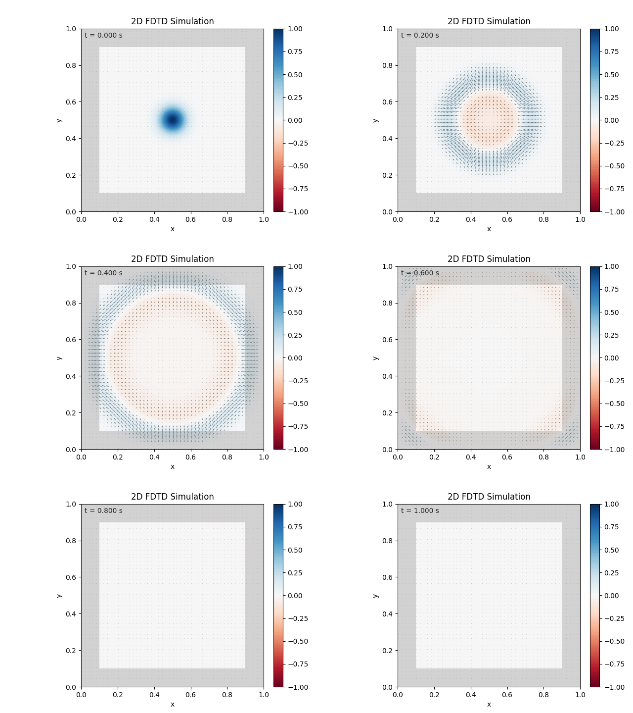
Tested with the same free-space setup as before:

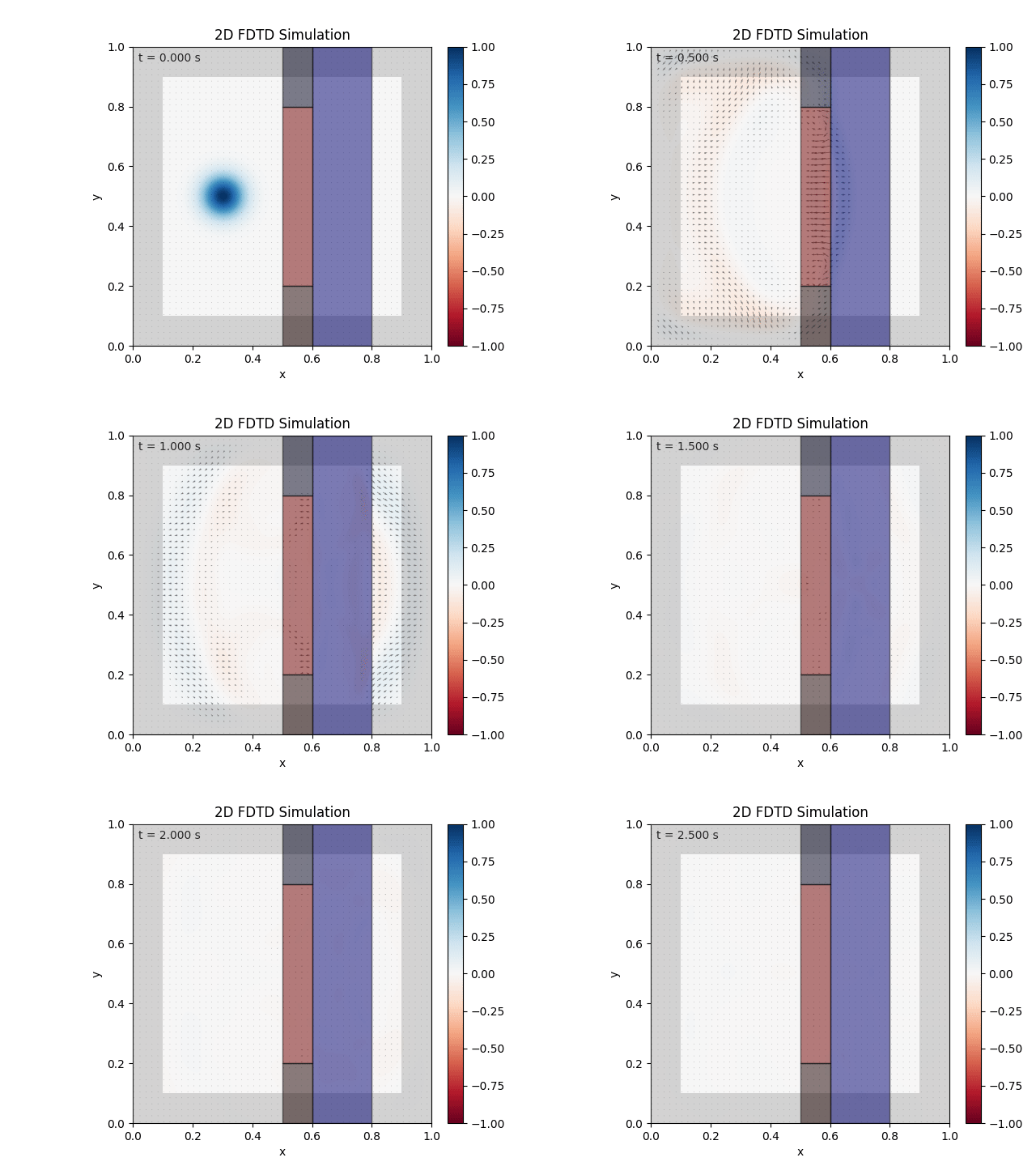
Looks like the PML is functioning. Testing materials:

Good work. Time to retire.