Theory
Consider the TDSE:
where $|\psi\rangle \coloneqq \psi(x,y,t)$ for this problem.
Expanding the Hamiltonian for non-relativistic particle:
Normalise and reduce dimensions ($\hbar = 2m = 1, \psi(x,y,t) \rightarrow u(x,y,t)$):
Noting also that $p(x,y,t)=u(x,y,t)\bar u(x,y,t)$ and that for all $t$,
The actual simulation can be done with the Crank-Nicolson method for PDEs (essentially just implicit Runge-Kutta). However, easier to approximate roughly with Euler/explicit Runge-Kutta.
We can do a simple rearrangement for the TSDE to get $\frac{\partial u}{\partial t}$ alone:
The 1D discrete Laplacian for a rectangular cuboid domain (i.e. row of simulation points) can be represented in matrix form as
Multidimensional discrete Laplacians on rectangular cuboid regular grids have very special properties, e.g., they are Kronecker sums of one-dimensional discrete Laplacians. (See: Kronecker sum of discrete Laplacians)
Therefore, we can construct the 2D ($N^2\times N^2$ matrix) representing the 2D version of the above using the Kronecker product:
setting $\mathbf L = \mathbf D_{\mathbf{xx}} \otimes \mathbf I_{\mathbf x} + \mathbf I_{\mathbf y} \otimes \mathbf D_{\mathbf{yy}}$ to be the 2D Laplacian where $\mathbf D_{\mathbf{xx}}$ is the 1D discrete Laplacian in the x-direction, etc. (Note that $\mathbf I_{\mathbf x},\mathbf I_{\mathbf y}$ has dimensions $N\times N$ for this problem.)
Whatever the Laplacian ends up being, we can ‘unroll’ $u_t(x,y)$ into a dimensionality $N^2$ vector, and applying the Hamiltonian on $u_t$ becomes matrix-vector multiplication.
Discretising and vectorizing with $u(x,y,t) \rightarrow \mathbf u_t$,
Details
Initial wavefunction was chosen to be a standard Gaussian wave packet, given by
For this project, Python was chosen since it’s the least hassle for implementation (Hint: I am still just bad at implementation)
The 2D Laplacian was computed with the following code:
def laplacian_2d(N):
	e = np.ones(N*N)
	L1D = np.diag(2*e) + np.diag(e[:-1], -1) + np.diag(e[1:], 1)
	L2D = np.kron(L1D, np.eye(N)) + np.kron(np.eye(N), L1D)
	return L2D
The Kronecker product is an expensive operation (by inspection $\mathcal O(N^4)$), but upon observation of the result, the 2D Laplacian (with Dirichlet boundary conditions) satisfies a very nice form (Hint: it does not in fact satisfy this nice form):
With this in mind we can optimise:
def laplacian_2d(N):
	e = np.ones(N*N)
	L2D = np.diag(-4*e) + np.diag(e[:-1], -1) + np.diag(e[1:], 1)
	return L2D
Unsurprisingly not only is this still slow ($\mathcal O(N^4)$) but also cannot support higher resolution grids ($N > 10^2$). With scipy.sparse however the time complexity can be significantly optimised:
def laplacian_2d(N):
	e = np.ones(N*N)
	L2D = sps.diags([-4*e, e[:-1], e[1:]], [0,-1,1], shape=(N*N, N*N),
		format='csr')
	return L2D
Construction is now $\mathcal O(N)$ since we add $\sim N$ non-zero entries.
Time evolution is just rewriting the discretisation into code:
def time_evolution(psi, V, dt):
	H = -1 * L2D + sps.diags(V.flatten(), 0, format='csr')
	psi_new = psi.flatten() - 1j * dt * H @ psi.flatten()
	return psi_new.reshape(N, N)
And for calling the function, save every save_interval steps since thousands of animation frames aren’t required and memory is saved so longer simulations can be run:
curr_psi = psi[0]
save_interval = 100

for i in range(int(T/dt)):
	if (i+1) % 100 == 0:
		print(f"Step {i+1}/{int(T/dt)}")
	psi_new = time_evolution(curr_psi, V, dt)
	psi_new[0, :] = psi_new[-1, :] = 0
	psi_new[:, 0] = psi_new[:, -1] = 0
	curr_psi = psi_new
	if (i+1) % save_interval == 0:
		psi.append(curr_psi)
Testing
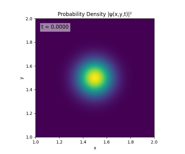
Instantiate an infinite potential square well and a Gaussian wavefunction in the centre, setting $L = 1.0, N=200,T=200,\Delta t=0.01$:
L = 1.0                 # domain size: [0,1]x[0,1]
N = 200                 # grid resolution
T = 100                 # final time
dt = 0.01               # time step
...
psi = []
V = np.zeros((N, N))
...
x = np.linspace(0, L, N)
y = np.linspace(0, L, N)
X, Y = np.meshgrid(x, y)
...
def init_psi(X, Y, x0, y0, sigma, px, py):
	norm = 1.0 / (sigma * np.sqrt(2 * np.pi))
	gauss = np.exp(- ((X - x0)**2 + (Y - y0)**2) / (4 * sigma**2))
	phase = np.exp(1j * (px * (X - x0) + py * (Y - y0)))
	psi.append(norm * gauss * phase)
And we obtain the following:
Clearly there are problems with the stability of the simulation. Below is plotted phase. Testing with $\Delta t=0.005$ shows that phase data gradually diverges and outstrips resolution (see left side).
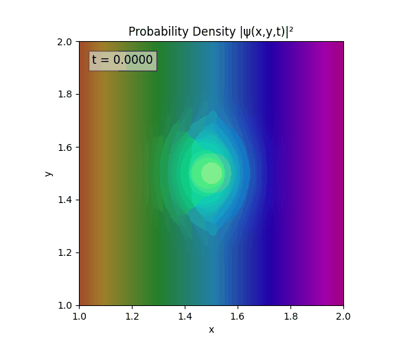
Not sure why - figure it’s something to do with the $\omega=5\pi$. Perhaps should downgrade a dimension first to check the theory is accurate (See: 1D TDSE simulation).
Removed explicit reinforcing of Dirichlet condition + speed optimisations (L2D.dot() instead of H @ psi) + adding the $\left( \frac{L}{N} \right)^2$ correction scalar on the Laplacian.

Clearly the Laplacian is incorrect, though the simulation already looks more stable. Didn’t notice the incorrect Laplacian since was explicitly reinforcing Dirichlet conditions anyway. I will switch back to a sparse Kronecker product:
def laplacian_2d(N):
	L1D = sps.diags([1, -2, 1], [-1, 0, 1], shape=(N, N), format='csr')
	L2D = sps.kron(L1D, sps.eye(N, format='csr'))
		+ sps.kron(sps.eye(N, format='csr'), L1D)
	L2D /= (L/N)**2
	return L2D
L2D = laplacian_2d(N)
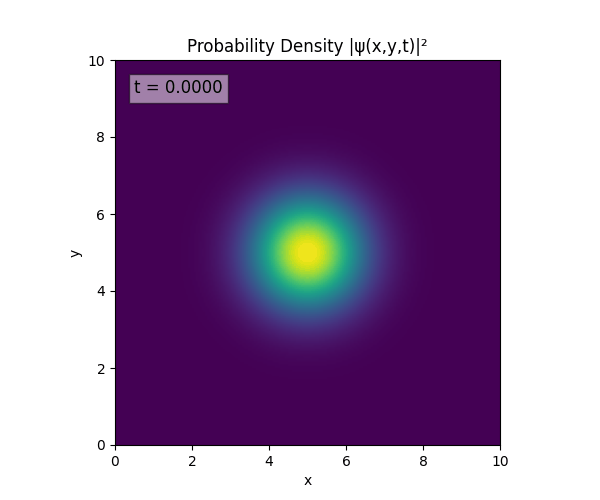
omg it works like the wave is expanding and it looks normal
Simulations
Code
import numpy as np
import scipy.integrate as spi
import scipy.sparse as sps
import matplotlib
import matplotlib.pyplot as plt
import matplotlib.animation as animation
INF = 1e10
# --- PARAMETERS ---
L = 10.0 # domain size: [0,1]x[0,1]
N = 200 # grid resolution
T = 2 # final time (adjust as needed)
dt = 0.01 # time step
def read_data():
det = open("sim.in", "r")
a, b = map(float, det.readline().split())
c, d = map(float, det.readline().split())
return a, int(b), c, d
L, N, T, dt = read_data()
# --- GRID ---
x = np.linspace(0, L, N)
y = np.linspace(0, L, N)
X, Y = np.meshgrid(x, y)
def init_psi(X, Y, x0, y0, sigma, px, py):
norm = 1.0 / (sigma * np.sqrt(2 * np.pi))
gauss = np.exp(- ((X - x0)**2 + (Y - y0)**2) / (4 * sigma**2))
phase = np.exp(1j * (px * (X - x0) + py * (Y - y0)))
return norm * gauss * phase
def well(X, Y):
V = np.zeros_like(X)
return V
# --- INITIALISE PSI/V ---
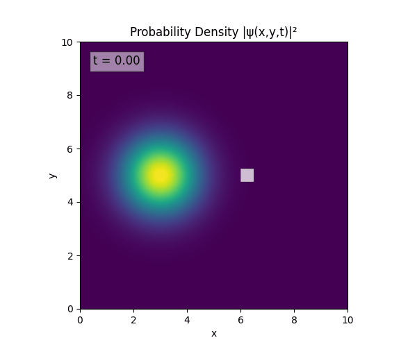
psi0 = init_psi(X, Y, 3, 5, 1, 2*np.pi, 0).flatten()
V = well(X, Y).flatten()
# --- CREATE LAPLACIAN OPERATOR ---
def laplacian_2d(N):
L1D = sps.diags([1, -2, 1], [-1, 0, 1], shape=(N, N), format='csr')
L2D = (sps.kron(L1D, sps.eye(N, format='csr')) + sps.kron(sps.eye(N, format='csr'), L1D)) / (L/N)**2
return L2D
L2D = laplacian_2d(N)
# --- TIME INTEGRATION ---
def dpsi_dt(t, psi):
psin = -1j * (-L2D.dot(psi) + V * psi)
return psin
sol = spi.solve_ivp(dpsi_dt, t_span=[0, T], y0=psi0, t_eval=np.arange(0, T, dt), method='RK23')
psi = sol.y.T.reshape(-1, N, N)
# --- VISUALISE ---
def create_visual():
fig, ax = plt.subplots(figsize=(6,5))
density = np.abs(psi[0])**2
im = ax.imshow(density, extent=[0, L, 0, L], origin='lower', cmap='viridis',
vmin=0, vmax=np.max(density), zorder=1)
cm_map = {
'red': ((0.0, 0.0, 0.0), (1.0, 1.0, 1.0)),
'green': ((0.0, 0.0, 0.0), (1.0, 1.0, 1.0)),
'blue': ((0.0, 0.0, 0.0), (1.0, 1.0, 1.0)),
'alpha': ((0.0, 0.0, 0.0), (1.0, 1.0, 1.0)),
}
v_map = matplotlib.colors.LinearSegmentedColormap('v_map', cm_map)
Vr = well(X, Y)
im2 = ax.imshow(Vr, extent=[0, L, 0, L], origin='lower', cmap=v_map,
vmin=0, vmax=np.max(Vr), zorder=2, alpha=0.75)
ax.set_xlabel('x')
ax.set_ylabel('y')
ax.set_title('Probability Density |ψ(x,y,t)|²')
time_txt = plt.text(0.05, 0.95, f't = {0:.2f}', transform=ax.transAxes,
fontsize=12, verticalalignment='top',
bbox=dict(facecolor='white', alpha=0.5), zorder=10)
def animate(i):
density = np.abs(psi[i])**2
im.set_data(density)
norm = matplotlib.cm.colors.Normalize(vmin=0, vmax=np.max(density))
im.set_norm(norm)
time_txt.set_text(f't = {(i*dt):.2f}')
return [im, im2, time_txt]
anim = animation.FuncAnimation(fig, animate, frames=len(psi), interval=50, blit=True, repeat=True)
anim.save('sim.gif', fps=10000, dpi=100)
plt.show()
create_visual()
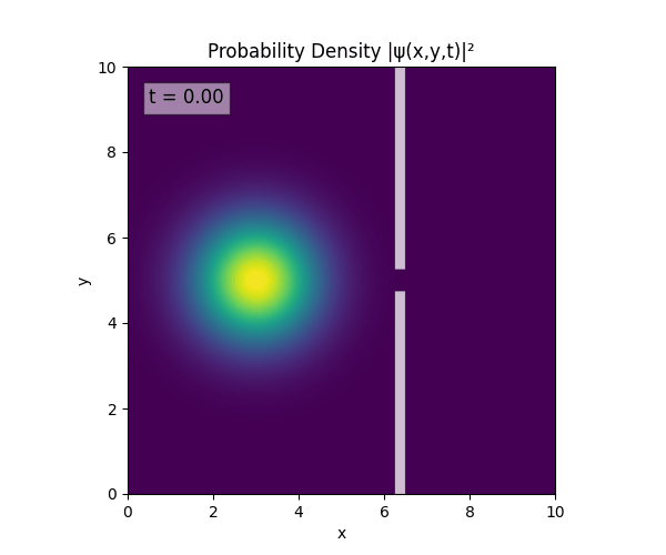
For all simulations, $L=10.0\text{ m},\,N=10^3,\,dt=0.01,\,T=1\text{ s}$ unless otherwise specified.
Reverse-Slit/Block ($T=1.5$)
Double Slit

Single Slit