Theory
Similar to the 2D TDSE setup:
Doing much the same theoretical setup ($\hbar=2m=1$):
And for this problem quite clearly $\nabla^2$ represented in matrix form as
The Gaussian wave-packet is
where $p_0$ is initial $x$ momentum.
Testing
import numpy as np
import scipy.integrate as spi
import scipy.linalg as spla
import scipy.sparse as sps
import matplotlib
import matplotlib.pyplot as plt
import matplotlib.animation as animation

INF = 1e10

# --- PARAMETERS ---

L = 1.0                 # domain size: [0,1]
N = 100                 # resolution
T = 5                   # final time
dt = 0.01              # time step

def read_data():
    det = open("sim.in", "r")
    a, b = map(float, det.readline().split())
    c, d = map(float, det.readline().split())
    return a, int(b), c, d
L, N, T, dt = read_data()

psi = []

# --- SPACE ---

x = np.linspace(0, L, N)

def init_psi(x, x0, sigma, p0):
    norm = 1.0 / (sigma * np.sqrt(2 * np.pi))
    gauss = np.exp(- (x - x0)**2 / (2 * sigma**2))
    phase = np.exp(1j * p0 * (x - x0))
    return norm * gauss * phase
def well(x):
    return np.zeros(N)

# --- INITIALISE PSI/V ---

psi = [init_psi(x, 5, 0.1, 2*np.pi)]
V = well(x)

# --- CREATE LAPLACIAN OPERATOR ---

def laplacian_1d(N):
    L1D = sps.diags([1, -2, 1], [-1, 0, 1], shape=(N, N), format='csr') / (L/N)**2
    return L1D
L1D = laplacian_1d(N)

# --- TIME INTEGRATION ---

def dpsi_dt(t, psi):
    H = -1 * L1D + sps.diags(V, 0, format='csr')
    psi_new = -1j * H @ psi
    # psi_new[0] = psi_new[-1] = 0
    return psi_new

sol = spi.solve_ivp(dpsi_dt, t_span=[0, T], y0=psi[0], t_eval=np.arange(0, T, dt), method='RK23')
psi = sol.y.T
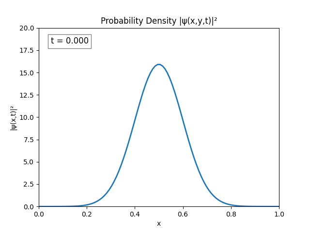
Unsurprisingly the same instability emerges. This could be because of resolution, both in terms of time and space ($dx,dt\to 0$ for perfect simulation), but this is untested since my program cannot run anything better than $dx=\frac{L}{N}=\frac{1}{100}\text{ m},\,dt=10^{-2}\text{ s}$.
After testing for various bugs I figured I could probably combat the issue just by increasing domain size, so that’s what I did.
Turns out performing the Dirichlet boundary conditions ($\psi(0)=\psi(t)=0$) explicitly is not necessary; the Laplacian does it automatically; and by not explicitly setting
psito 0, the peaks in the simulation disappear.
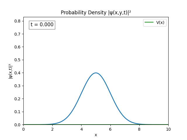
The simulation actually looks alright. I believe the only issue is $L = 1.0$ is too small since the wave spreads pretty quickly.
By increasing $L = 10.0\text{ m}$ while retaining $\frac{L}{N}=10^{-2}\implies N=1000$, we obtain:
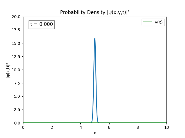
I’m not sure that this is correct. Hint: Turns out it’s correct.
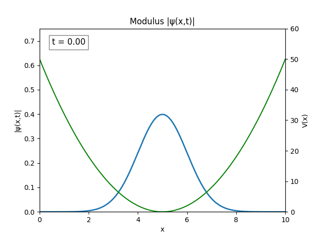
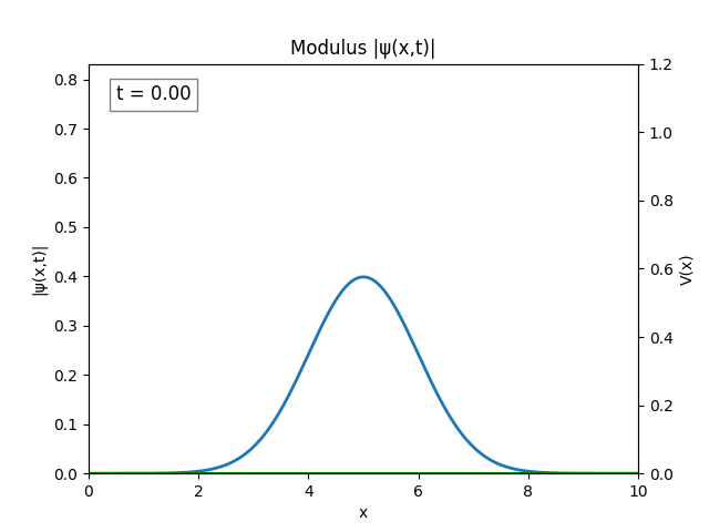
The wave spreading can be controlled by setting $\sigma$ to be larger, say $\sigma=1$. Graphing the modulus of the wave gives a nice result.
I’m happy with this so I’ll try a couple potential functions and then call this project.
Simulations
Code
import numpy as np
import scipy.integrate as spi
import scipy.linalg as spla
import scipy.sparse as sps
import matplotlib
import matplotlib.pyplot as plt
import matplotlib.animation as animation

INF = 1e10

# --- PARAMETERS ---

L = 10.0                # domain size: [0,1]
N = 1000                # resolution
T = 2                   # final time
dt = 0.01               # time step

def read_data():
    det = open("sim.in", "r")
    a, b = map(float, det.readline().split())
    c, d = map(float, det.readline().split())
    return a, int(b), c, d
L, N, T, dt = read_data()

# --- SPACE ---

x = np.linspace(0, L, N)

def init_psi(x, x0, sigma, p0):
    norm = 1.0 / (sigma * np.sqrt(2 * np.pi))
    gauss = np.exp(- (x - x0)**2 / (2 * sigma**2))
    phase = np.exp(1j * p0 * (x - x0))
    return norm * gauss * phase
def well(x):
    return np.zeros(N)

# --- INITIALISE PSI/V ---

psi0 = init_psi(x, 3, 1, 2*np.pi)
V = well(x)

# --- CREATE LAPLACIAN OPERATOR ---

def laplacian_1d(N):
    L1D = sps.diags([1, -2, 1], [-1, 0, 1], shape=(N, N), format='csr') / (L/N)**2
    return L1D
L1D = laplacian_1d(N)

# --- TIME INTEGRATION ---

def dpsi_dt(t, psi):
    return -1j * (-L1D.dot(psi) + V * psi)

sol = spi.solve_ivp(dpsi_dt, t_span=[0, T], y0=psi0, t_eval=np.arange(0, T, dt), method='RK23')
psi = sol.y.T

# --- VISUALISE ---

def create_visual():
    fig, ax = plt.subplots()
    all = np.array(abs(psi)).flatten()
    ax.set_xlim(0, L)
    ax.set_ylim(0, 1.2 * np.max(all))
    line, = ax.plot([], [], lw=2)
    ax.set_xlabel('x')
    ax.set_ylabel('|ψ(x,t)|')
    ax.set_title('Modulus |ψ(x,t)|')

    ax2 = ax.twinx()
    ax2.set_ylim(0, 1.2 * max(np.max(V), 1))
    ax2.set_ylabel('V(x)')
    well_line, = ax2.plot(x, V, label="V(x)", color="green")

    density = np.abs(psi[0])
    line.set_data(x, density)

    time_txt = plt.text(0.05, 0.95, f't = {0:.2f}', transform=ax.transAxes,
                        fontsize=12, verticalalignment='top',
                        bbox=dict(facecolor='white', alpha=0.5), zorder=10)

    def animate(i):
        density = np.abs(psi[i])
        line.set_data(x, density)
        time_txt.set_text(f't = {i*dt:.2f}')
        return [line, time_txt]

    anim = animation.FuncAnimation(fig, animate, frames=len(psi), interval=50, blit=True)
    anim.save('sim.gif', fps=120, dpi=100)

    plt.show()

create_visual()
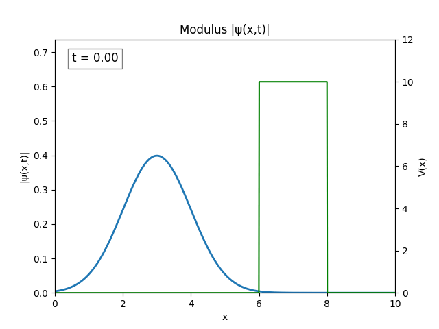
For all simulations, $L=10.0\text{ m},\,N=10^3,\,dt=0.01,\,T=2\text{ s}$ unless otherwise specified.
Infinite Square Well
Heaviside
Funny Well ($T=5$)